# setwd('C:/R-Project/DAT/Regression/')chapter 3, chapter 4
library(ggplot2)Data
dt <- data.frame(x = c(4,8,9,8,8,12,6,10,6,9),
                 y = c(9,20,22,15,17,30,18,25,10,20))
dt| x | y |
|---|---|
| <dbl> | <dbl> |
| 4 | 9 |
| 8 | 20 |
| 9 | 22 |
| 8 | 15 |
| 8 | 17 |
| 12 | 30 |
| 6 | 18 |
| 10 | 25 |
| 6 | 10 |
| 9 | 20 |
correlation check
cor(dt$x, dt$y)
0.921812343945765
산점도 확인
plot(y~x,
     data = dt,
     xlab = "광고료",
     ylab = "총판매액",
     pch  = 16,
     cex  = 2,
     col  = "darkorange")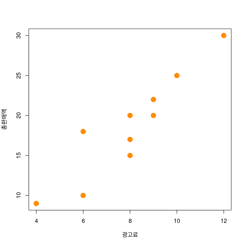
pch 점 모양
cex 점 크기
양의상관관계 강하네,
우상향이네, 단순상관선형 적용해보면 되겠다.
ggplot(dt, aes(x, y)) +
  geom_point(col='steelblue', lwd=2) +
  # geom_abline(intercept = co[1], slope = co[2], col='darkorange', lwd=1.2) +
  xlab("광고료")+ylab("총판매액")+
  # scale_x_continuous(breaks = seq(1,10))+
  theme_bw() +
  theme(axis.title = element_text(size = 14))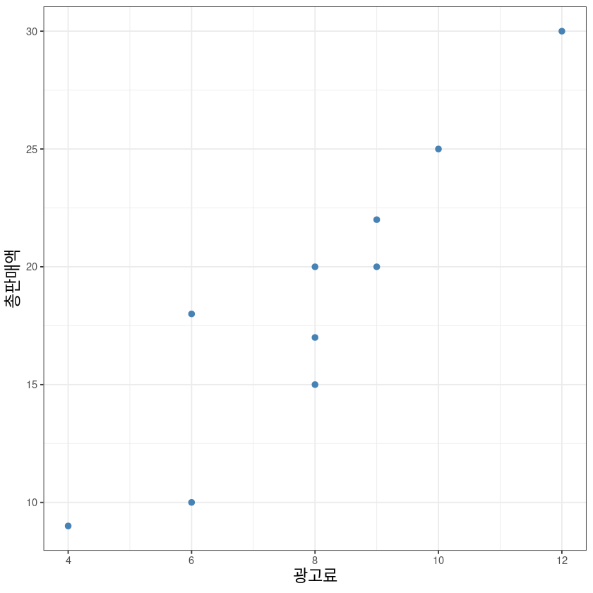
적합
\(\hat{ y} = \widehat{(E(y|X=x))} = \hat{\beta_0} + \hat{\beta_1} * x\)
\(H_0\) : \(\beta_0\) =0 vs \(H_1\) : \(\beta_0 \ne 0\)
\(H_0\) : \(\beta_1 =0\) vs \(H_1\) : \(\beta_1 \ne 0\)
모형 적합을 한다 yhat을 찾는다. - 회귀분석을 한다. 평균 반응을 추정한다.
lm linear model 사용
## y = beta0 + beta1*x + epsilon
model1 <- lm(y ~ x, dt)
# lm(y ~ 0 + x, dt) beta0 없이 분석하고 싶을때
model1
Call:
lm(formula = y ~ x, data = dt)

Coefficients:
(Intercept)            x
     -2.270        2.609
설명변수 x 하나일때
- beta0hat = -2.270
- beta1hat = 2.609
summary(model1)
Call:
lm(formula = y ~ x, data = dt)

Residuals:
   Min     1Q Median     3Q    Max
-3.600 -1.502  0.813  1.128  4.617

Coefficients:
            Estimate Std. Error t value Pr(>|t|)
(Intercept)  -2.2696     3.2123  -0.707 0.499926
x             2.6087     0.3878   6.726 0.000149 ***
---
Signif. codes:  0 ‘***’ 0.001 ‘**’ 0.01 ‘*’ 0.05 ‘.’ 0.1 ‘ ’ 1

Residual standard error: 2.631 on 8 degrees of freedom
Multiple R-squared:  0.8497,    Adjusted R-squared:  0.831
F-statistic: 45.24 on 1 and 8 DF, p-value: 0.0001487- 모형의 유의성 검정 자체(f검정)
- 개별 회귀계수에 대한 유의성검정(t검정)
- beta1은 유의하지 않다
- beta0는 유의하다
- f통계량은 45.24(msr/mse) p값 충분히 작아서 모형은 유의하다.
- y의 총 변동 중에 85%정도를 설명하고 있다.
- root mse(RMSE) = 2.631
6.726**2
45.239076
단순선형에서만 해당
0.000149도 같음
names(model1)- 'coefficients'
- 'residuals'
- 'effects'
- 'rank'
- 'fitted.values'
- 'assign'
- 'qr'
- 'df.residual'
- 'xlevels'
- 'call'
- 'terms'
- 'model'
model1$residuals # 보고 싶은 변수 입력해봐~- 1
- 0.834782608695656
- 2
- 1.4
- 3
- 0.791304347826087
- 4
- -3.6
- 5
- -1.6
- 6
- 0.96521739130435
- 7
- 4.61739130434782
- 8
- 1.18260869565217
- 9
- -3.38260869565218
- 10
- -1.20869565217391
model1$fitted.values  ##hat y
model1$coefficients- 1
- 8.16521739130434
- 2
- 18.6
- 3
- 21.2086956521739
- 4
- 18.6
- 5
- 18.6
- 6
- 29.0347826086957
- 7
- 13.3826086956522
- 8
- 23.8173913043478
- 9
- 13.3826086956522
- 10
- 21.2086956521739
- (Intercept)
- -2.2695652173913
- x
- 2.60869565217391
anova(model1) ## 회귀모형의 유의성 검정| Df | Sum Sq | Mean Sq | F value | Pr(>F) | |
|---|---|---|---|---|---|
| <int> | <dbl> | <dbl> | <dbl> | <dbl> | |
| x | 1 | 313.04348 | 313.043478 | 45.24034 | 0.0001486582 |
| Residuals | 8 | 55.35652 | 6.919565 | NA | NA |
- 설명변수의 개수가 x 자유도
- 잔차의 자유도는 n-2
a <- summary(model1)
ls(a)- 'adj.r.squared'
- 'aliased'
- 'call'
- 'coefficients'
- 'cov.unscaled'
- 'df'
- 'fstatistic'
- 'r.squared'
- 'residuals'
- 'sigma'
- 'terms'
summary(model1)$coef ## 회귀계수의 유의성 검정| Estimate | Std. Error | t value | Pr(>|t|) | |
|---|---|---|---|---|
| (Intercept) | -2.269565 | 3.212348 | -0.7065129 | 0.4999255886 |
| x | 2.608696 | 0.387847 | 6.7260939 | 0.0001486582 |
confint(model1, level = 0.95)  ##회귀계수의 신뢰구간
## beta +- t_alpha/2 (n-2) * se(beta)
qt(0.025, 8)
qt(0.975, 8)| 2.5 % | 97.5 % | |
|---|---|---|
| (Intercept) | -9.677252 | 5.138122 |
| x | 1.714319 | 3.503073 |
-2.30600413520417
2.30600413520417
- qt _ tquantile
## y = beta1*x + epsilon
model2 <- lm(y ~ 0 + x, dt)
summary(model2)
Call:
lm(formula = y ~ 0 + x, data = dt)

Residuals:
    Min      1Q  Median      3Q     Max
-4.0641 -1.5882  0.2638  1.4818  3.9359

Coefficients:
  Estimate Std. Error t value Pr(>|t|)
x   2.3440     0.0976   24.02  1.8e-09 ***
---
Signif. codes:  0 ‘***’ 0.001 ‘**’ 0.01 ‘*’ 0.05 ‘.’ 0.1 ‘ ’ 1

Residual standard error: 2.556 on 9 degrees of freedom
Multiple R-squared:  0.9846,    Adjusted R-squared:  0.9829
F-statistic: 576.8 on 1 and 9 DF, p-value: 1.798e-09- intercept 없는 모습
- r squre가 두 번째가 높고,
- p값도 훨씬 유의하게 나옴
anova(model1)| Df | Sum Sq | Mean Sq | F value | Pr(>F) | |
|---|---|---|---|---|---|
| <int> | <dbl> | <dbl> | <dbl> | <dbl> | |
| x | 1 | 313.04348 | 313.043478 | 45.24034 | 0.0001486582 |
| Residuals | 8 | 55.35652 | 6.919565 | NA | NA |
anova(model2)| Df | Sum Sq | Mean Sq | F value | Pr(>F) | |
|---|---|---|---|---|---|
| <int> | <dbl> | <dbl> | <dbl> | <dbl> | |
| x | 1 | 3769.1895 | 3769.1895 | 576.8138 | 1.79763e-09 |
| Residuals | 9 | 58.8105 | 6.5345 | NA | NA |
###########
plot(y~x, data = dt,
     xlab = "광고료",
     ylab = "총판매액",
     pch  = 20,
     cex  = 2,
     col  = "darkorange")
abline(model1, col='steelblue', lwd=2)
abline(model2, col='green', lwd=2)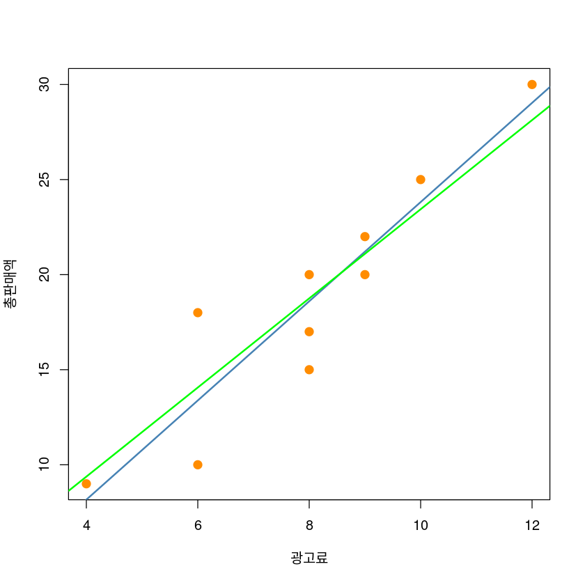
model들이 기울기가 살짝씩 다르다
co <- coef(model1)ggplot(dt, aes(x, y)) +
geom_point(col='steelblue', lwd=1) +
geom_abline(intercept = co[1], slope = co[2], col='darkorange', lwd=1) +
xlab("광고료")+ylab("총판매액")+
theme_bw()+
theme(axis.title = element_text(size = 16))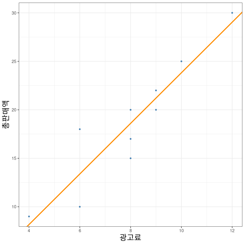
######## LSE 구하기
# lm을 사용하지 않고 구할때

dt1 <- data.frame(
  i = 1:nrow(dt),
  x = dt$x,
  y = dt$y,
  x_barx = dt$x - mean(dt$x), # x - x평균
y_bary = dt$y - mean(dt$y)) # y - y평균dt1$x_barx2 <- dt1$x_barx^2 # x 편차의 제곱
dt1$y_bary2 <- dt1$y_bary^2 # y편차의 제곱
dt1$xy <-dt1$x_barx * dt1$y_barydt1| i | x | y | x_barx | y_bary | x_barx2 | y_bary2 | xy |
|---|---|---|---|---|---|---|---|
| <int> | <dbl> | <dbl> | <dbl> | <dbl> | <dbl> | <dbl> | <dbl> |
| 1 | 4 | 9 | -4 | -9.6 | 16 | 92.16 | 38.4 |
| 2 | 8 | 20 | 0 | 1.4 | 0 | 1.96 | 0.0 |
| 3 | 9 | 22 | 1 | 3.4 | 1 | 11.56 | 3.4 |
| 4 | 8 | 15 | 0 | -3.6 | 0 | 12.96 | 0.0 |
| 5 | 8 | 17 | 0 | -1.6 | 0 | 2.56 | 0.0 |
| 6 | 12 | 30 | 4 | 11.4 | 16 | 129.96 | 45.6 |
| 7 | 6 | 18 | -2 | -0.6 | 4 | 0.36 | 1.2 |
| 8 | 10 | 25 | 2 | 6.4 | 4 | 40.96 | 12.8 |
| 9 | 6 | 10 | -2 | -8.6 | 4 | 73.96 | 17.2 |
| 10 | 9 | 20 | 1 | 1.4 | 1 | 1.96 | 1.4 |
round(colSums(dt1),3)- i
- 55
- x
- 80
- y
- 186
- x_barx
- 0
- y_bary
- 0
- x_barx2
- 46
- y_bary2
- 368.4
- xy
- 120
### hat beta1 = S_xy / S_xx
##hat beta0 = bar y - hat beta_1 * bar x
beta1 <- as.numeric(colSums(dt1)[8]/colSums(dt1)[6])
beta0 <- mean(dt$y) - beta1 * mean(dt$x)cat("hat beta0 = ", beta0)
cat("hat beta1 = ", beta1)hat beta0 = -2.269565hat beta1 = 2.608696평균반응, 개별 y 추정
구분할 수 있어야 한다
신뢰구간 달라진다.
## E(Y|x0) 평균반응
## y = E(Y|x0) + epsilon 개별 y 추정
# x0 = 4.5
new_dt <- data.frame(x = 4.5)
# hat y0 = hat beta0 + hat beta1 * 4.5
predict(model1,
newdata = new_dt,
interval = c("confidence"), level = 0.95)| fit | lwr | upr | |
|---|---|---|---|
| 1 | 9.469565 | 5.79826 | 13.14087 |
new_data=new_df 정의 안 하면 fitted value가 나온다.
confidence는 평균반응
predict(model1, newdata = new_dt,
interval = c("prediction"), level = 0.95)| fit | lwr | upr | |
|---|---|---|---|
| 1 | 9.469565 | 2.379125 | 16.56001 |
prediction은 개별 y 추정
신뢰구간이 커진다. \(\to\) 표준오차가 달라지기 때문
dt_pred <- data.frame(
  x = 1:12,
  predict(model1,
          newdata=data.frame(x=1:12),
          interval="confidence", level = 0.95))
dt_pred| x | fit | lwr | upr | |
|---|---|---|---|---|
| <int> | <dbl> | <dbl> | <dbl> | |
| 1 | 1 | 0.3391304 | -6.2087835 | 6.887044 |
| 2 | 2 | 2.9478261 | -2.7509762 | 8.646628 |
| 3 | 3 | 5.5565217 | 0.6905854 | 10.422458 |
| 4 | 4 | 8.1652174 | 4.1058891 | 12.224546 |
| 5 | 5 | 10.7739130 | 7.4756140 | 14.072212 |
| 6 | 6 | 13.3826087 | 10.7597808 | 16.005437 |
| 7 | 7 | 15.9913043 | 13.8748223 | 18.107786 |
| 8 | 8 | 18.6000000 | 16.6817753 | 20.518225 |
| 9 | 9 | 21.2086957 | 19.0922136 | 23.325178 |
| 10 | 10 | 23.8173913 | 21.1945634 | 26.440219 |
| 11 | 11 | 26.4260870 | 23.1277880 | 29.724386 |
| 12 | 12 | 29.0347826 | 24.9754543 | 33.094111 |
dt_pred2 <- as.data.frame(predict(model1,
                                  newdata=data.frame(x=1:12),
                                  interval="prediction", level = 0.95))
dt_pred2| fit | lwr | upr | |
|---|---|---|---|
| <dbl> | <dbl> | <dbl> | |
| 1 | 0.3391304 | -8.5867330 | 9.264994 |
| 2 | 2.9478261 | -5.3751666 | 11.270819 |
| 3 | 5.5565217 | -2.2199297 | 13.332973 |
| 4 | 8.1652174 | 0.8663128 | 15.464122 |
| 5 | 10.7739130 | 3.8692308 | 17.678595 |
| 6 | 13.3826087 | 6.7738957 | 19.991322 |
| 7 | 15.9913043 | 9.5667143 | 22.415894 |
| 8 | 18.6000000 | 12.2379683 | 24.962032 |
| 9 | 21.2086957 | 14.7841056 | 27.633286 |
| 10 | 23.8173913 | 17.2086783 | 30.426104 |
| 11 | 26.4260870 | 19.5214047 | 33.330769 |
| 12 | 29.0347826 | 21.7358781 | 36.333687 |
names(dt_pred2)[2:3] <- c('plwr', 'pupr')plot 같이 그리게 데이터 합치기
dt_pred3 <- cbind.data.frame(dt_pred, dt_pred2[,2:3])barx <- mean(dt$x)
bary <- mean(dt$y)plot(y~x, data = dt,
xlab = "광고료",
ylab = "총판매액",
pch = 20,
cex = 2,
col = "grey",
ylim = c(min(dt_pred3$plwr), max(dt_pred3$pupr)))
abline(model1, lwd = 5, col = "darkorange")
lines(dt_pred3$x, dt_pred3$lwr, col = "dodgerblue", lwd = 3, lty = 2)
lines(dt_pred3$x, dt_pred3$upr, col = "dodgerblue", lwd = 3, lty = 2)
lines(dt_pred3$x, dt_pred3$plwr, col = "dodgerblue", lwd = 3, lty = 3)
lines(dt_pred3$x, dt_pred3$pupr, col = "dodgerblue", lwd = 3, lty = 3)
abline(h=bary,v=barx, lty=2, lwd=0.2, col='dark grey')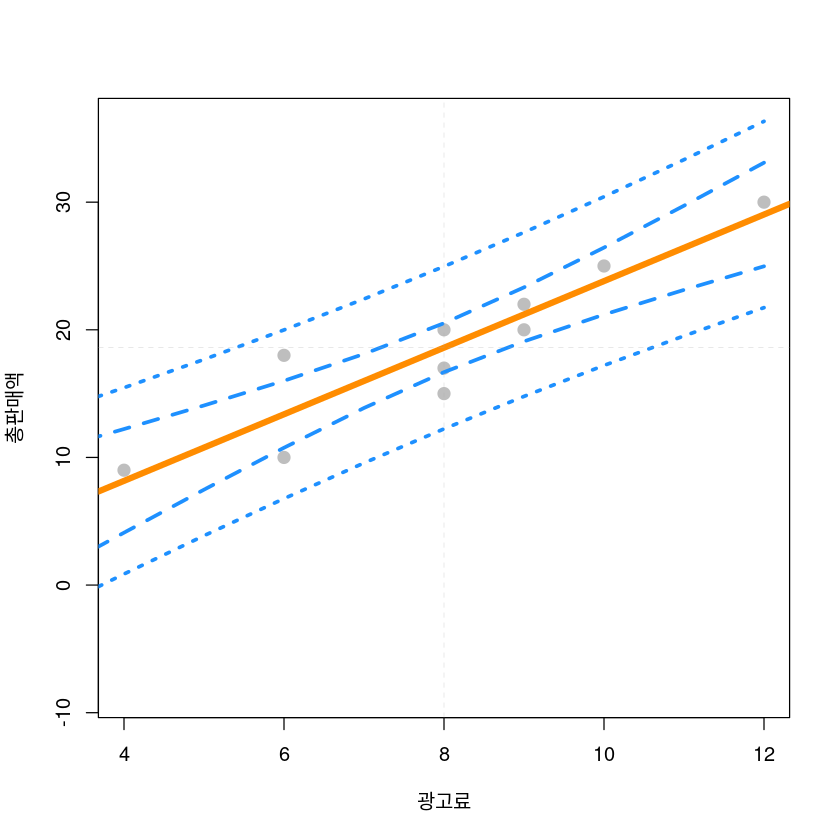
ggplot(dt_pred3, aes(x, fit)) +
  geom_line(col='steelblue', lwd=2) +
  xlab("")+ylab("")+
  scale_x_continuous(breaks = seq(1,10))+
  geom_line(aes(x, lwr), lty=2, lwd=1.5, col='darkorange') +
  geom_line(aes(x, upr), lty=2, lwd=1.5, col='darkorange') +
  geom_line(aes(x, plwr), lty=2, lwd=1.5, col='dodgerblue') +
  geom_line(aes(x, pupr), lty=2, lwd=1.5, col='dodgerblue') +
  geom_vline(xintercept = barx, lty=2, lwd=0.2, col='dark grey')+
  geom_hline(yintercept = bary, lty=2, lwd=0.2, col='dark grey')+
  theme_bw()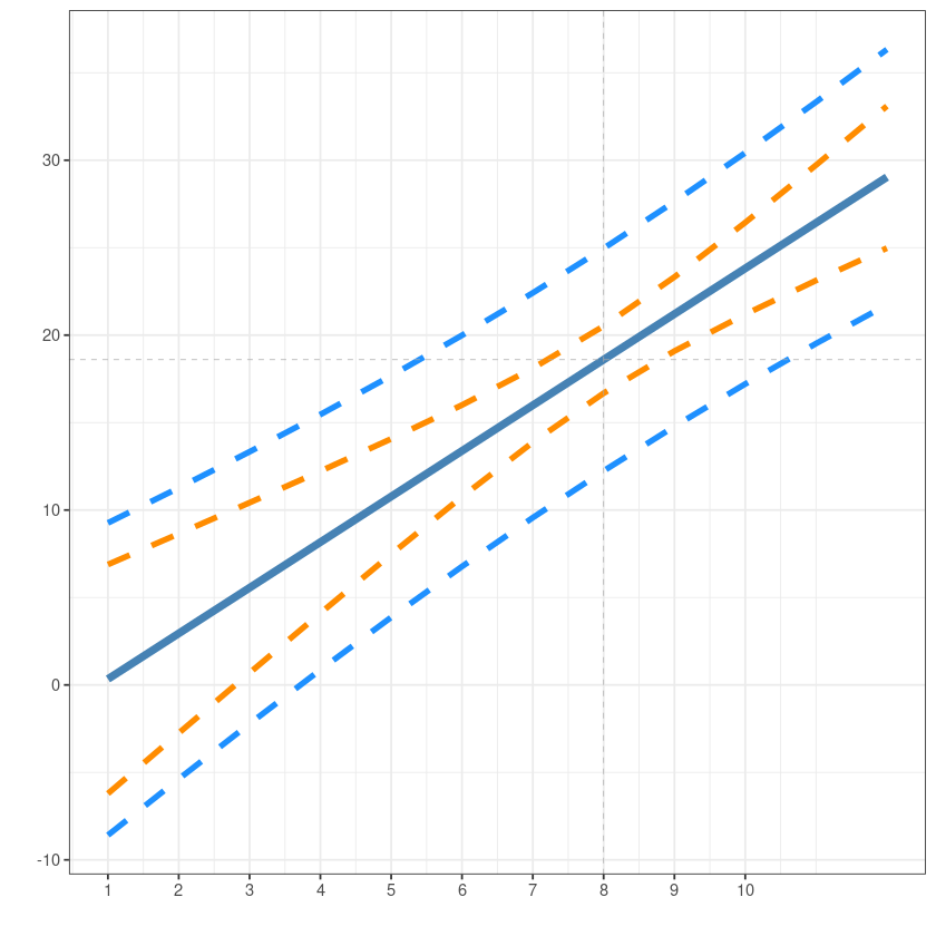
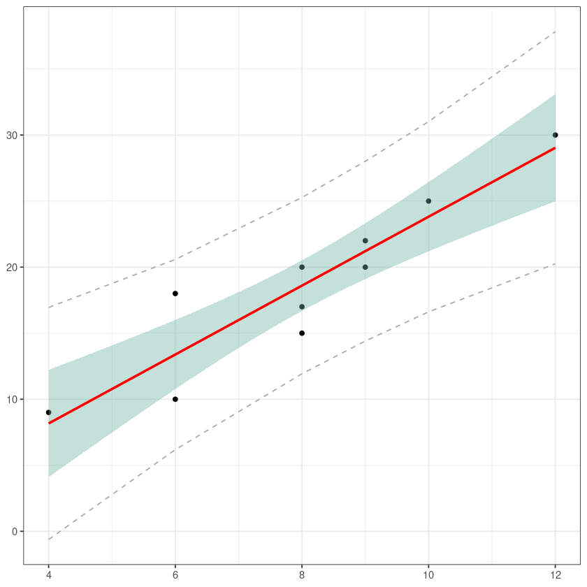
bb <- summary(model1)$sigma * ( 1 + 1/10 +(dt$x - 8)^2/46)
dt$ma95y <- model1$fitted + 2.306*bb
dt$mi95y <- model1$fitted - 2.306*bbggplot(dt, aes(x=x, y=y)) +
geom_point() +
geom_smooth(method=lm , color="red", fill="#69b3a2", se=TRUE) +
geom_line(aes(x, mi95y), col = 'darkgrey', lty=2) +
geom_line(aes(x, ma95y), col = 'darkgrey', lty=2) +
theme_bw() +
theme(axis.title = element_blank())`geom_smooth()` using formula 'y ~ x'
잔차분석
### epsilon : 선형성, 등분산성, 정규성, 독립성dt
dt$yhat <- model1$fitted
# fitted.values(model1) # y에 대한 추정값 구하기
dt$resid <- model1$residuals
# resid(model1)| x | y | ma95y | mi95y |
|---|---|---|---|
| <dbl> | <dbl> | <dbl> | <dbl> |
| 4 | 9 | 16.94766 | -0.6172208 |
| 8 | 20 | 25.27254 | 11.9274568 |
| 9 | 22 | 28.01311 | 14.4042841 |
| 8 | 15 | 25.27254 | 11.9274568 |
| 8 | 17 | 25.27254 | 11.9274568 |
| 12 | 30 | 37.81722 | 20.2523444 |
| 6 | 18 | 20.58263 | 6.1825918 |
| 10 | 25 | 31.01741 | 16.6173744 |
| 6 | 10 | 20.58263 | 6.1825918 |
| 9 | 20 | 28.01311 | 14.4042841 |
par(mfrow=c(1,2))
plot(resid ~ x, dt, pch=16, ylab = 'Residual')
abline(h=0, lty=2, col='grey')
plot(resid ~ yhat, dt, pch=16, ylab = 'Residual')
abline(h=0, lty=2, col='grey')
par(mfrow=c(1,1))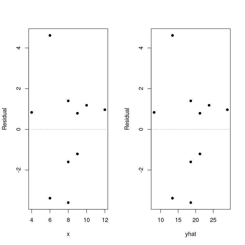
단순선형에서는 두 plot의 차이가 없다.
- 선형성 만족
- 등분산성 나름 만족
- 정규성 아웃라이어 있는 거 같은데..
- 독립성?
# 독립성검정 : DW test
library(lmtest)
Loading required package: zoo
Attaching package: ‘zoo’
The following objects are masked from ‘package:base’:
as.Date, as.Date.numeric
##
dwtest(model1, alternative = "two.sided")  #H0 : uncorrelated vs H1 : rho != 0
# dwtest(model1, alternative = "greater")  #H0 : uncorrelated vs H1 : rho > 0
# dwtest(model1, alternative = "less")  #H0 : uncorrelated vs H1 : rho < 0
    Durbin-Watson test

data:  model1
DW = 1.4679, p-value = 0.3916
alternative hypothesis: true autocorrelation is not 0
p 값 커서 기각할 수 없다.
첫 번째꺼 주로 보기
## 정규분포 (QQ plot)
qqnorm(dt$resid, pch=16)
qqline(dt$resid, col = 2)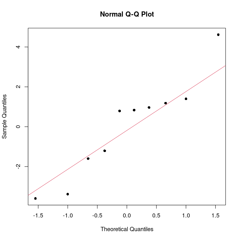
분위수분위수 그림 - 정규분포의 실제 - 어떤 분포의 이론적 분위수와 내가 가진 sample의 분위수 비교
주로 꼬리쪽을 많이 본다. - 이 데이터의 경우 꼬리부분이 차이가 커 보임
ggplot(dt, aes(sample = resid)) +
  stat_qq() + stat_qq_line() +
  theme_bw()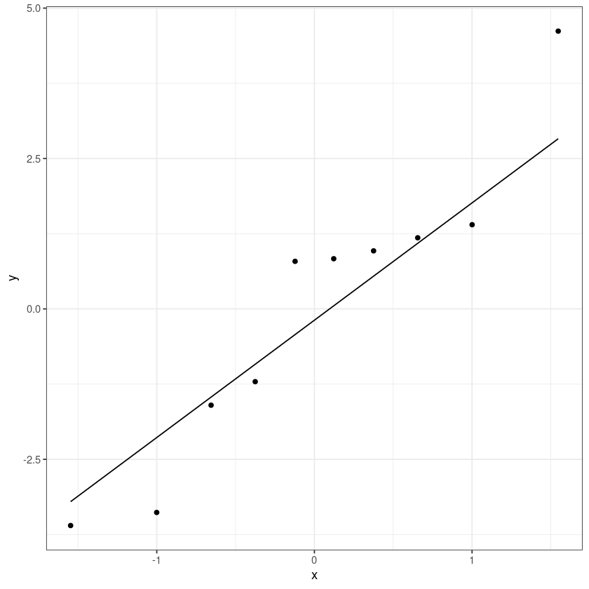
## 정규분포 검정
shapiro.test(dt$resid)  ##shapiro-wilk test
#H0 : normal distributed vs H1 : not
    Shapiro-Wilk normality test

data:  dt$resid
W = 0.92426, p-value = 0.3939
p값 작게 나오면 정규분포라고 하기 어렵다.
- 정규성은 잔차를 넣어줬는데
- bptest는 model을 넣었다.
## 등분산성 검정
bptest(model1) #Breusch–Pagan test
# H0 : 등분산 vs H1 : 이분산
    studentized Breusch-Pagan test

data:  model1
BP = 1.6727, df = 1, p-value = 0.1959
책 예제
# install.packages('UsingR')
library(UsingR)
Loading required package: MASS
Loading required package: HistData
Loading required package: Hmisc
Loading required package: lattice
Loading required package: survival
Loading required package: Formula
Attaching package: ‘Hmisc’
The following objects are masked from ‘package:base’:
format.pval, units
Attaching package: ‘UsingR’
The following object is masked from ‘package:survival’:
cancer
data(father.son)names(father.son)- 'fheight'
- 'sheight'
lm.fit<-lm(sheight~fheight, data=father.son)summary(lm.fit)
Call:
lm(formula = sheight ~ fheight, data = father.son)

Residuals:
    Min      1Q  Median      3Q     Max
-8.8772 -1.5144 -0.0079  1.6285  8.9685

Coefficients:
            Estimate Std. Error t value Pr(>|t|)
(Intercept) 33.88660    1.83235   18.49   <2e-16 ***
fheight      0.51409    0.02705   19.01   <2e-16 ***
---
Signif. codes:  0 ‘***’ 0.001 ‘**’ 0.01 ‘*’ 0.05 ‘.’ 0.1 ‘ ’ 1

Residual standard error: 2.437 on 1076 degrees of freedom
Multiple R-squared:  0.2513,    Adjusted R-squared:  0.2506
F-statistic: 361.2 on 1 and 1076 DF,  p-value: < 2.2e-16
아버지의 키가 아들의 키의 25%만 설명
plot(sheight~fheight,
     data=father.son,
     pch=16, cex=0.5,
     xlab="father’s height (inches)",
     ylab="son’s height (inches)")
abline(lm.fit)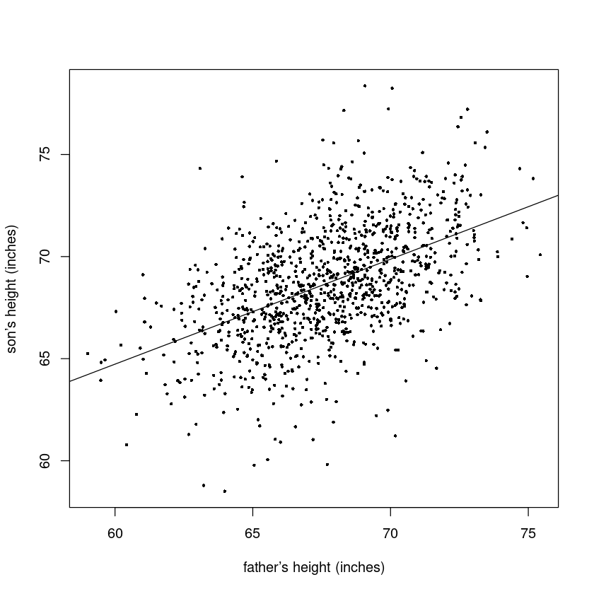
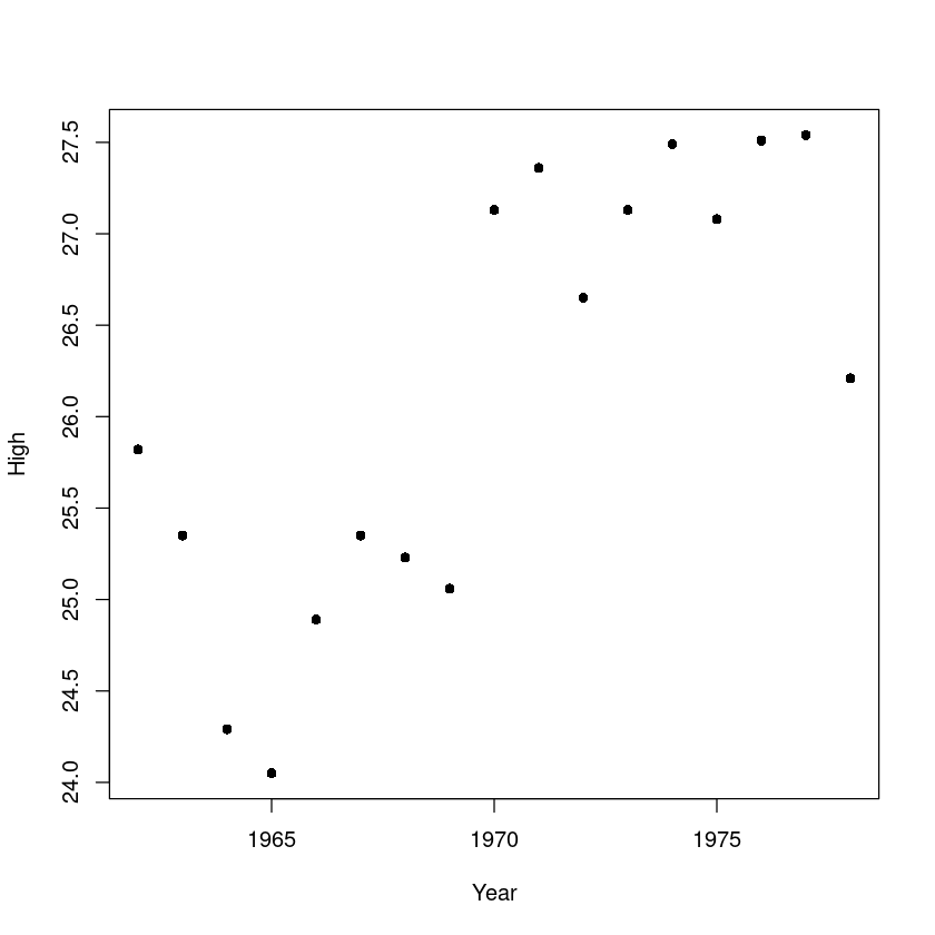
amazon<-read.csv("amazon.csv")
plot(High   ~Year  , amazon, pch=16)

lm.fit<-lm(High~Year, data=amazon)
summary(lm.fit)

confint(lm.fit)

par(mfrow=c(1,2))
scatter.smooth(x=1:length(amazon$Year), y=residuals(lm.fit), xlab="Year")
scatter.smooth(x=predict(lm.fit), y=residuals(lm.fit), xlab=expression(hat(y)))

library(lmtest)
dwtest(lm.fit)
Call:
lm(formula = High ~ Year, data = amazon)

Residuals:
    Min      1Q  Median      3Q     Max
-1.3629 -0.5341  0.1479  0.4903  1.1412

Coefficients:
              Estimate Std. Error t value Pr(>|t|)
(Intercept) -330.21235   78.03319  -4.232 0.000725 ***
Year           0.18088    0.03961   4.567 0.000371 ***
---
Signif. codes:  0 ‘***’ 0.001 ‘**’ 0.01 ‘*’ 0.05 ‘.’ 0.1 ‘ ’ 1

Residual standard error: 0.8001 on 15 degrees of freedom
Multiple R-squared:  0.5816,    Adjusted R-squared:  0.5537
F-statistic: 20.85 on 1 and 15 DF, p-value: 0.0003708| 2.5 % | 97.5 % | |
|---|---|---|
| (Intercept) | -496.53615985 | -163.8885460 |
| Year | 0.09645429 | 0.2653104 |
    Durbin-Watson test

data:  lm.fit
DW = 1.0487, p-value = 0.006864
alternative hypothesis: true autocorrelation is greater than 0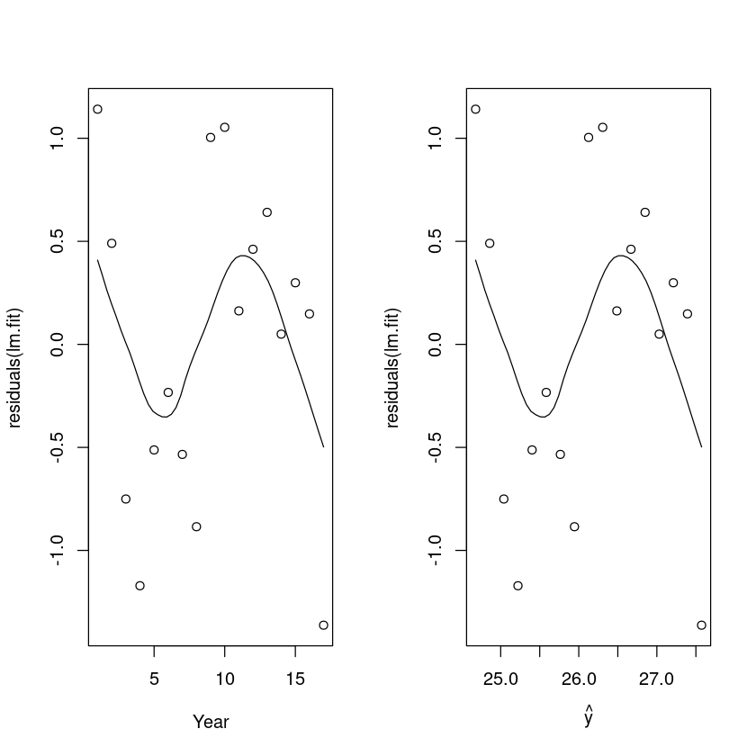
양의 상관관계가 있다. - 시간순 index - 최근 관측 데이터에 영향 많이 받는 편